

Image Processing 101 Chapter 2.2: Point Operations
This post discusses the basic point operations and the next post will be covering spatial filters.
Point Operation
Point operations are often used to change the grayscale range and distribution. The concept of point operation is to map every pixel onto a new image with a predefined transformation function.
g(x, y) = T(f(x, y))
- g (x, y) is the output image
- T is an operator of intensity transformation
- f (x, y) is the input image
Basic Intensity Transformation Functions
The simplest image enhancement method is to use a 1 x 1 neighborhood size. It is a point operation. In this case, the output pixel (‘s’) only depends on the input pixel (‘r’), and the point operation function can be simplified as follows:
s = T(r)
Where T is the point operator of a certain gray-level mapping relationship between the original image and the output image.
- s,r: denote the gray level of the input pixel and the output pixel.
Different transformation functions work for different scenarios.
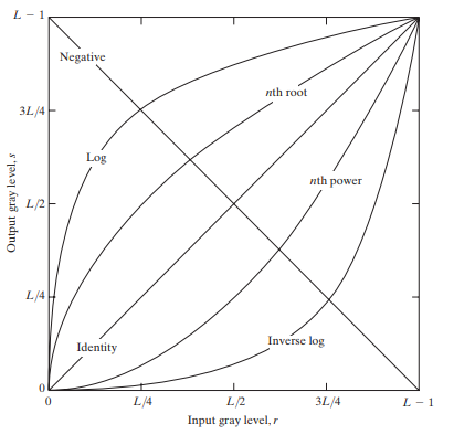
Image source: Slideshare.net
Linear
Linear transformations include identity transformation and negative transformation.
In identity transformation, the input image is the same as the output image.
s = r
The negative transformation is:
s = L - 1 - r = 256 - 1 - r = 255 - r
L = Largest gray level in an image. The negative transformation is suited for enhancing white or gray detail embedded in dark areas of an image, for example, analyzing the breast tissue in a digital mammogram.
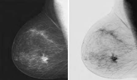
Image source: Slideshare.net
Logarithmic
a) General Log Transform
The equation of general log transformation is:
s = c * log(1 + r)
Note:
- s,r: denote the gray level of the input pixel and the output pixel.
- ‘c’ is a constant; to map from [0,255] to [0,255], c = 255/LOG(256)
- the base of a common logarithm is 10
In the log transformation, the low-intensity values are mapped into higher intensity values. It maps a narrow range of low gray levels to a much wider range. Generally speaking, the log transformation works the best for dark images.
Image source: Slideshare.net
b) Inverse Log Transform
The inverse log transform is opposite to log transform. It maps a narrow range of high gray levels to a much wider range. The inverse log transform expands the values of light-level pixels while compressing the darker-level values.
s = power(10, r * c)-1
Note:
- s,r: denote the gray level of the input pixel and the output pixel.
- ‘c’ is a constant; to map from [0,255] to [0,255], c =LOG(256)/255
Power-Law (Gamma) Transformation
The gamma transform, also known as exponential transformation or power transformation, is a commonly used grayscale non-linear transformation. The mathematical expression of the gamma transformation is as follows:
s = c * power(r, γ), where
- s,r: denote the gray level of the input pixel and the output pixel;
- ‘c’ is a constant
- ‘γ’ is also a constant and is the gamma coefficient.
Plots of the equation [formula] for various values of γ (c = 1 in all cases)
All curves were scaled to fit in the range shown. X-axis represents input intensity level ‘r’, and y-axis represents the output intensity level ‘s’.
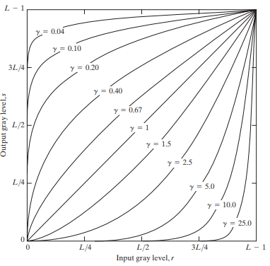
Image source: Slideshare.net
When performing the conversion, it is a common practice to first convert the intensity level from the range of 0 to 255 to 0 to 1. Then perform the gamma conversion and at last restore to the original range.
Comparing to log transformation, gamma transformation can generate a family of possible transformation curves by varying the gamma value.
Here are the enhanced images output by using different γ (gamma) values.
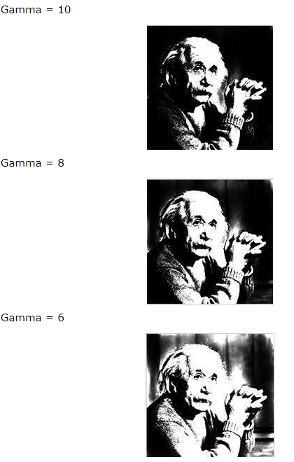
Image source: TutorialsPoint.com
The gamma transformation can selectively enhance the contrast of the dark region or the light region depending on the value of γ.
- When γ > 1, the contrast of the light gray area is enhanced. Take γ = 25 for example, the pixels with the range of 0.8-1 (at the scale of 256, it corresponds to 240-255) are mapped to the range of 0-1
- When γ < 1, the contrast of the dark gray area is enhanced
- When γ = 1, this transformation is linear, that is, the original image is not changed
Piecewise Transformation
In mathematics, a piecewise-defined function is a function defined by multiple sub-functions, where each sub-function applies to a different interval in the domain. ※
Types of piecewise transformations:
- Grayscale Threshold Transform (Gray-level Slicing)
- Contrast Stretching
- Bit-plane Slicing
Grayscale Threshold Transform
Grayscale Threshold Transform converts a grayscale image into a black and white binary image. The user specifies a value that acts as a dividing line. If the gray value of a pixel is smaller than the dividing, the intensity of the pixel is set to 0, otherwise it’s set to 255. The value of the dividing line is called the threshold. The grayscale threshold transform is often referred to as thresholding, or binarization.

Contrast-Stretching Transformation
The goal of the contrast-stretching transformation is to enhance the contrast between different parts of an image, that is, enhances the gray contrast for areas of interest, and suppresses the gray contrast for areas that are not of interest.
Below are two possible functions:
1. Power-Law Contrast-Stretching Transformation
If T(r) has the form as shown in the figure, the effect of applying the transformation to every pixel to generate the corresponding pixels produce higher contrast than the original image, by:
- Darkening the levels below k in the original image
- Brightening the levels above k in the original image

2. Linear Contrast-Stretching Transformation
Points (r1, s1) and (r2, s2) control the shape of the transformation. The selection of control points depends upon the types of image and varies from one image to another image. If r1 = s1 and r2 = s2 then the transformation is linear and this doesn’t affect the image. In other case we can calculate the intensity of output pixel, provided intensity of input pixel is x, as follows:
- For 0 <= x <= r1 output = s1 / r1 * x
- For r1 < x <= r2 output = ((s2 – s1)/(r2 – r1))*(x – r1) + s1
- For r2 < x <= L-1 output = ((L-1 – s2)/(L-1 – r2))*(x – r2) + s2

Bit-plane Slicing
As discussed previously, each pixel of a grayscale image is stored as a 8-bit byte. The intensity spans from 0 to 255, which is ‘00000000’ to ‘11111111’ in binary.
Bit-plane slicing refers to the process of slicing a matrix of 8 bits into 8 planes.
The most left bit (the 8th bit from right to left) carries the most weight so it is called the Most Signification Bit. The most right bit (the 1st bit from right to left) carries the least weight so it is called the Least Signification Bit.
Advanced: Histogram Equalization
Histogram equalization, also known as grayscale equalization, is a practical histogram correction technique.
It refers to the transformation where an output image has approximately the same number of pixels at each gray level, i.e., the histogram of the output is uniformly distributed. In the equalized image, the pixels will occupy as many gray levels as possible and be evenly distributed. Therefore, such image has a higher contrast ratio and a larger dynamic range.
This method is to boost the global contrast of an image to make it look more visible.
The general histogram equalization formula is:
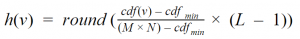
- CDF refers to the cumulative distribution function
- L is the maximum intensity value (typically 256)
- M is the image width and N is the image height
- h (v) is the equalized value
Before Histogram Equalization 🠕

Histogram Chart Before Equalization 🠕
After Histogram Equalization 🠕

Histogram Chart After Equalization 🠕
This article is Part 5 in a 7-Part Series.
- Part 1 - Image Processing 101 Chapter 1.1: What is an Image?
- Part 2 - Image Processing 101 Chapter 1.2: Color Models
- Part 3 - Image Processing 101 Chapter 1.3: Color Space Conversion
- Part 4 - Image Processing 101 Chapter 2.1: Image Enhancement
- Part 5 - Image Processing 101 Chapter 2.2: Point Operations
- Part 6 - Image Processing 101 Chapter 2.3: Spatial Filters (Convolution)
- Part 7 - Morphological Operations