


Image Smoothing & Sharpening in Image Processing using Spatial Filters
In the last post, we discussed gamma transformation, histogram equalization, and other image enhancement techniques. The commonality of these methods is that the transformation is directly related to the pixel gray value, independent of the neighborhood in which the pixel is located.
In this post, we take a look at the spatial domain enhancement where neighborhood pixels are also used.
A General Concept
The spatial domain enhancement is based on pixels in a small range (neighbor). This means the transformed intensity is determined by the gray values of those points within the neighborhood, and thus the spatial domain enhancement is also called neighborhood operation or neighborhood processing.
A digital image can be viewed as a two-dimensional function f (x, y), and the x-y plane indicates spatial position information, called the spatial domain. The filtering operation based on the x-y space neighborhood is called spatial domain filtering.
Spatial filtering with a template
The filtering process is to move the filter point-by-point in the image function f (x, y) so that the center of the filter coincides with the point (x, y). At each point (x, y), the filter’s response is calculated based on the specific content of the filter and through a predefined relationship called ‘template’.
If the pixel in the neighborhood is calculated as a linear operation, it is also called ‘linear spatial domain filtering’, otherwise, it’s called ‘nonlinear spatial domain filtering’. Figure 2.3.1 shows the process of spatial filtering with a 3 × 3 template (also known as a filter, kernel, or window).
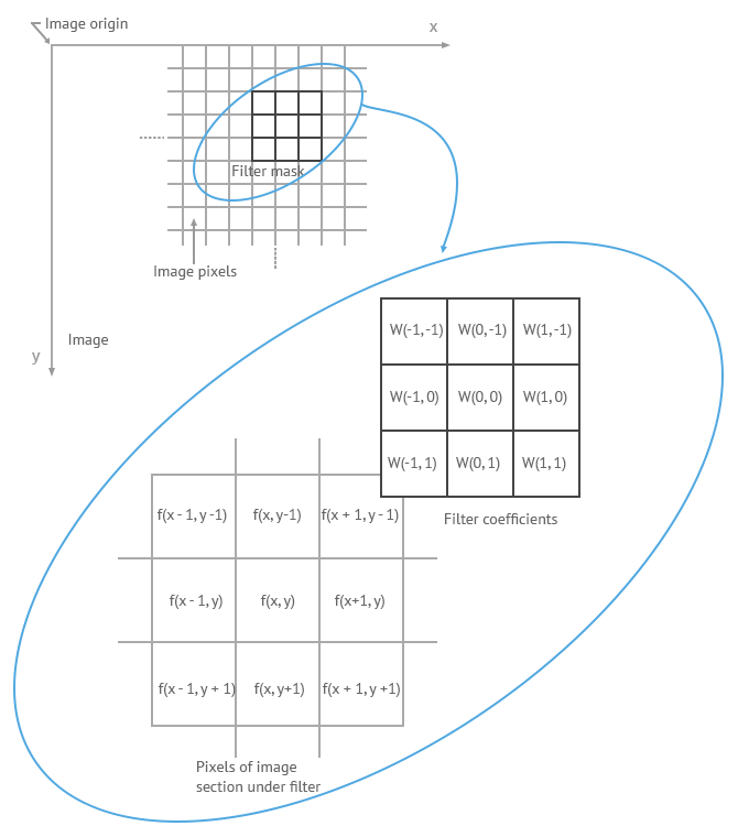
Figure 2.3.1
The coefficients of the filter in linear spatial filtering give a weighting pattern. For example, for Figure 2.3.1, the response ‘R’ to the template is:
R = w(-1, -1) * f (x-1, y-1) + w(-1, 0) * f (x-1, y) + …+ w( 0, 0) * f (x, y) +…+ w(1, 0) * f (x+1, y) + w (1, 1) * f( x+1, y+1)
In mathematics, this is known as element-wise matrix multiplication. For a filter with a size of (2a+1, 2b+1), the output response can be calculated with the following function:
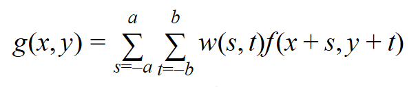
In the following, we will take a look at the filters of image smoothing and sharpening.
Smoothing Filters
Image smoothing is a digital image processing technique that reduces and suppresses image noises. In the spatial domain, neighborhood averaging can generally be used to achieve the purpose of smoothing. Commonly seen smoothing filters include average smoothing, Gaussian smoothing, and adaptive smoothing.
Average Smoothing
First, let’s take a look at the smoothing filter in its simplest form — average template and its implementation.
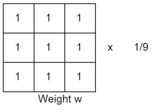
The points in the 3 × 3 neighborhood centered on the point (x, y) are altogether involved in determining the (x, y) point pixel in the new image ‘g’. All coefficients being 1 means that they contribute the same (weight) in the process of calculating the g(x, y) value. The last coefficient, 1/9, is to ensure that the sum of the entire template elements is 1. This keeps the new image in the same grayscale range as the original image (e.g., [0, 255]). Such a ‘w’ is called an average template.
How it works?
In general, the intensity values of adjacent pixels are similar, and the noise causes grayscale jumps at noise points. However, it is reasonable to assume that occasional noises do not change the local continuity of an image. Take the image below for example, there are two dark points in the bright area.
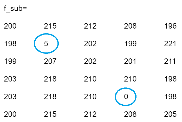
For the borders, we can add a padding using the “replicate” approach. When smoothing the image with a 3×3 average template, the resulting image is the following.
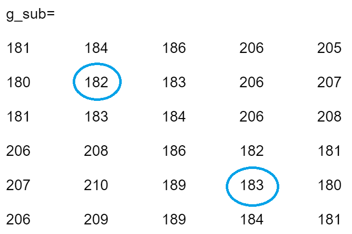
The two noises are replaced with the average of their surrounding points. The process of reducing the influence of noise is called smoothing or blurring.
Gaussian Smoothing
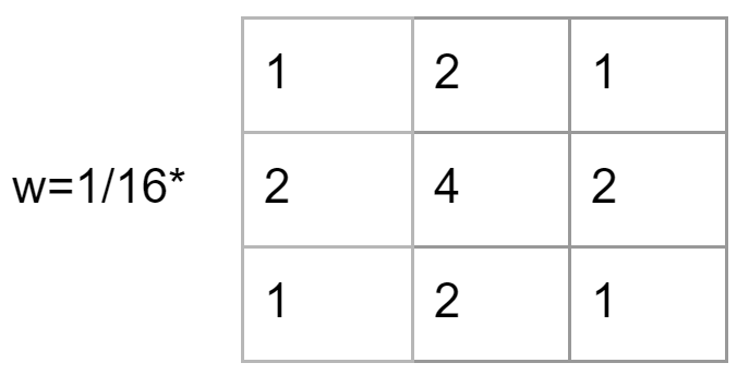
The average smoothing treats the same to all the pixels in the neighborhood. In order to reduce the blur in the smoothing process and obtain a more natural smoothing effect, it is natural to think to increase the weight of the template center point and reduce the weight of distant points. So that the new center point intensity is closer to its nearest neighbors. The Gaussian template is based on such consideration.
The commonly used 3 × 3 Gaussian template is shown below.
Adaptive Smoothing
The average template blurs the image while eliminating the noise. Gaussian template does a better job, but the blurring is still inevitable as it’s rooted in the mechanism. A more desirable way is selective smoothing, that is, smoothing only in the noise area, and not smoothing in the noise-free area. This way potentially minimizes the influence of the blur. It is called adaptive filtering.
So how to determine if the local area needs to be smoothed with noise? The answer lies in the nature of the noise, that is, the local continuity. The presence of noise causes a grayscale jump at the noise point, thus making a large grayscale span. Therefore, one of the following two can be used as the criterion:
- The difference between the maximum intensity and the minimum intensity of a local area is greater than a certain threshold T, ie: max(R) – min(R) > T, where R represents the local area.
- The variance is greater than a certain threshold T, i.e, D(R) > T, where D(R) represents the variance of the pixels in the area R.
Others
There are some other approaches to tackle the smoothing, such as median filter and adaptive median filter.
Sharpening Filters
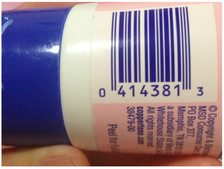
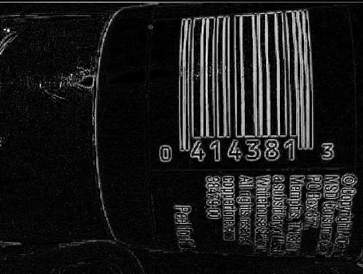
Image sharpening filters highlight edges by removing blur. It enhances the grayscale transition of an image, which is the opposite of image smoothing. The arithmetic operators of smoothing and sharpening also testifies the fact. While linear smoothing is based on the weighted summation or integral operation on the neighborhood, the sharpening is based on the derivative (gradient) or finite difference.
How to distinguish noises and edges still matters in sharpening. The difference is that, in smoothing we try to smooth noise and ignore edges and in sharpening we try to enhance edges and ignore noise.
Some applications of where sharpening filters are used include:
- Medical image visualization
- Photo enhancement
- Industrial defect detection
- Autonomous guidance in military systems
There are a couple of filters that can be used for sharpening. One of the most popular filters is Laplace operator. It is based on second order differential.
The corresponding filter template is as follows:
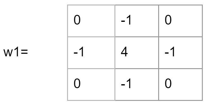
With the sharpening enhancement, two numbers with the same absolute value represent the same response, so w1 is equivalent to the following template w2:
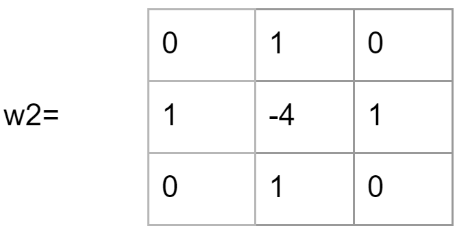
Taking a further look at the structure of the Laplacian template, we see that the template is isotropic for a 90-degree rotation. Laplace operator performs well for edges in the horizontal direction and the vertical direction, thus avoiding the hassle of having to filter twice.
Example
This article is Part 6 in a 7-Part Series.
- Part 1 - Image Processing 101 Chapter 1.1: What is an Image?
- Part 2 - Image Processing 101 Chapter 1.2: Understanding Color Models and Their Uses
- Part 3 - Color Space Conversion & Binarization for Image Processing
- Part 4 - Image Processing 101 Chapter 2.1: A Complete Guide to Enhancing Visual Quality
- Part 5 - Point Operations in Image Processing: A Beginner's Guide
- Part 6 - Image Smoothing & Sharpening in Image Processing using Spatial Filters
- Part 7 - Morphological Operations